Chapter 12 Regularization
Chapter Status: Currently this chapter is very sparse. It essentially only expands upon an example discussed in ISL, thus only illustrates usage of the methods. Mathematical and conceptual details of the methods will be added later.
We will use the Hitters dataset from the ISLR package to explore two shrinkage methods: ridge regression and lasso. These are otherwise known as penalized regression methods.
This dataset has some missing data in the response Salaray. We use the na.omit() function to clean the dataset for ease-of-use.
## [1] 59## [1] 59## [1] 0The feature variables are offensive and defensive statistics for a number of baseball players.
##  [1] "AtBat"     "Hits"      "HmRun"     "Runs"      "RBI"       "Walks"
##  [7] "Years"     "CAtBat"    "CHits"     "CHmRun"    "CRuns"     "CRBI"
## [13] "CWalks"    "League"    "Division"  "PutOuts"   "Assists"   "Errors"
## [19] "Salary"    "NewLeague"
We use the glmnet() and cv.glmnet() functions from the glmnet package to fit penalized regressions.
Unfortunately, the glmnet function does not allow the use of model formulas, so we setup the data for ease of use with glmnet. Eventually we will use train() from caret which does allow for fitting penalized regression with the formula syntax, but to explore some of the details, we first work with the functions from glmnet directly.
Note, we’re being lazy and just using the full dataset as the training dataset.
First, we fit an ordinary linear regression, and note the size of the features’ coefficients, and features’ coefficients squared. (The two penalties we will use.)
##  (Intercept)        AtBat         Hits        HmRun         Runs          RBI
##  163.1035878   -1.9798729    7.5007675    4.3308829   -2.3762100   -1.0449620
##        Walks        Years       CAtBat        CHits       CHmRun        CRuns
##    6.2312863   -3.4890543   -0.1713405    0.1339910   -0.1728611    1.4543049
##         CRBI       CWalks      LeagueN    DivisionW      PutOuts      Assists
##    0.8077088   -0.8115709   62.5994230 -116.8492456    0.2818925    0.3710692
##       Errors   NewLeagueN
## -3.3607605 -24.7623251## [1] 238.7295## [1] 18337.312.1 Ridge Regression
We first illustrate ridge regression, which can be fit using glmnet() with alpha = 0 and seeks to minimize
\[ \sum_{i=1}^{n} \left( y_i - \beta_0 - \sum_{j=1}^{p} \beta_j x_{ij} \right) ^ 2 + \lambda \sum_{j=1}^{p} \beta_j^2 . \]
Notice that the intercept is not penalized. Also, note that that ridge regression is not scale invariant like the usual unpenalized regression. Thankfully, glmnet() takes care of this internally. It automatically standardizes predictors for fitting, then reports fitted coefficient using the original scale.
The two plots illustrate how much the coefficients are penalized for different values of \(\lambda\). Notice none of the coefficients are forced to be zero.
par(mfrow = c(1, 2))
fit_ridge = glmnet(X, y, alpha = 0)
plot(fit_ridge)
plot(fit_ridge, xvar = "lambda", label = TRUE)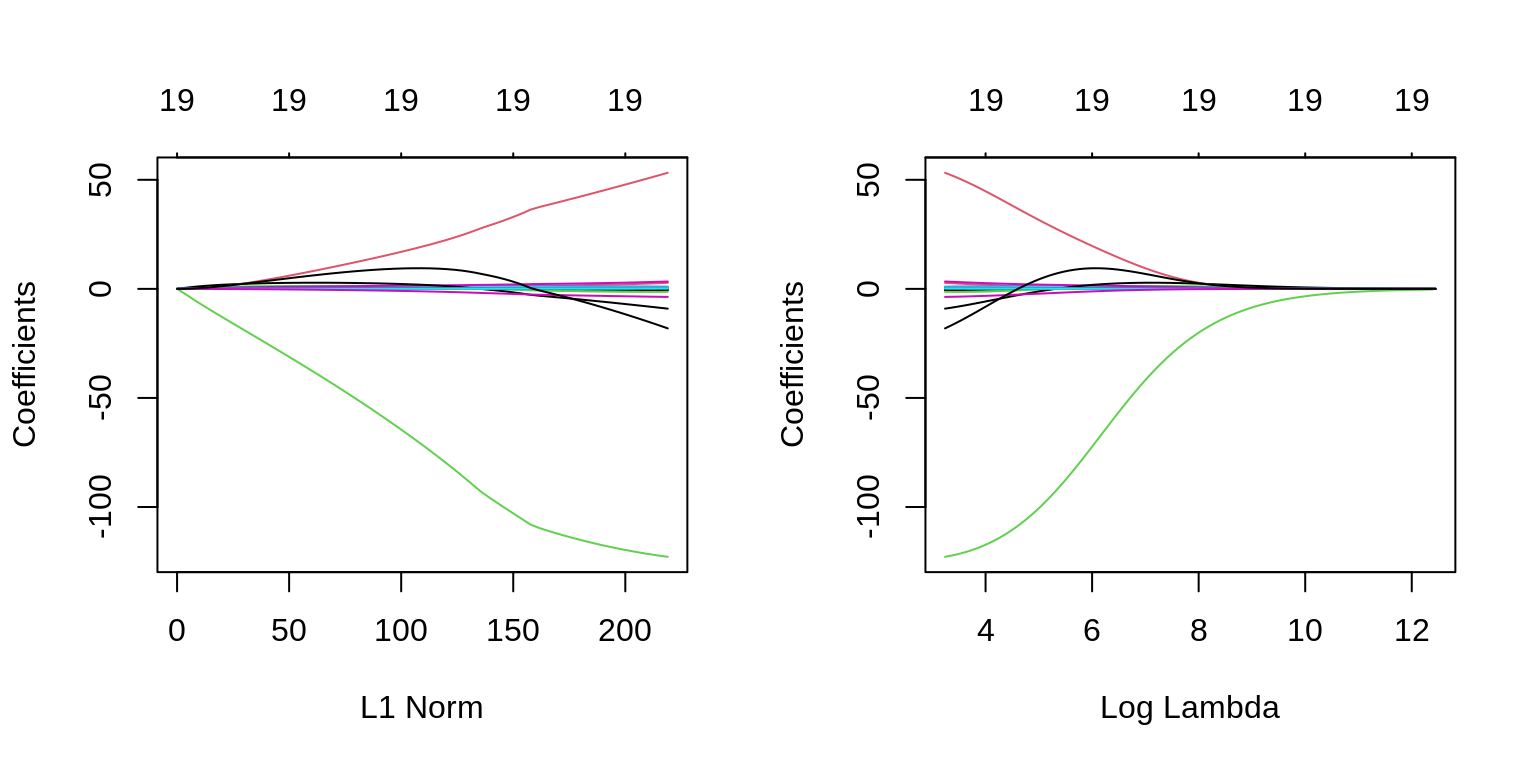
We use cross-validation to select a good \(\lambda\) value. The cv.glmnet()function uses 10 folds by default. The plot illustrates the MSE for the \(\lambda\)s considered. Two lines are drawn. The first is the \(\lambda\) that gives the smallest MSE. The second is the \(\lambda\) that gives an MSE within one standard error of the smallest.
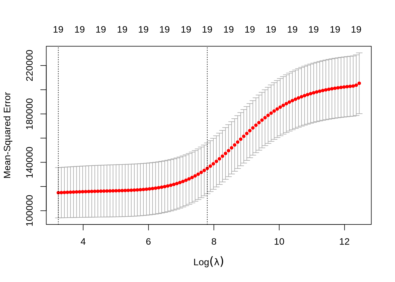
The cv.glmnet() function returns several details of the fit for both \(\lambda\) values in the plot. Notice the penalty terms are smaller than the full linear regression. (As we would expect.)
## 20 x 1 sparse Matrix of class "dgCMatrix"
##                         1
## (Intercept) 199.418113624
## AtBat         0.093426871
## Hits          0.389767263
## HmRun         1.212875007
## Runs          0.623229048
## RBI           0.618547529
## Walks         0.810467707
## Years         2.544170910
## CAtBat        0.007897059
## CHits         0.030554662
## CHmRun        0.226545984
## CRuns         0.061265846
## CRBI          0.063384832
## CWalks        0.060720300
## LeagueN       3.743295031
## DivisionW   -23.545192292
## PutOuts       0.056202373
## Assists       0.007879196
## Errors       -0.164203267
## NewLeagueN 3.313773161## 20 x 1 sparse Matrix of class "dgCMatrix"
## 1
## (Intercept) 8.112693e+01
## AtBat -6.815959e-01
## Hits 2.772312e+00
## HmRun -1.365680e+00
## Runs 1.014826e+00
## RBI 7.130225e-01
## Walks 3.378558e+00
## Years -9.066800e+00
## CAtBat -1.199478e-03
## CHits 1.361029e-01
## CHmRun 6.979958e-01
## CRuns 2.958896e-01
## CRBI 2.570711e-01
## CWalks -2.789666e-01
## LeagueN 5.321272e+01
## DivisionW -1.228345e+02
## PutOuts 2.638876e-01
## Assists 1.698796e-01
## Errors -3.685645e+00
## NewLeagueN -1.810510e+01## [1] 18367.29## 20 x 1 sparse Matrix of class "dgCMatrix"
## 1
## (Intercept) 199.418113624
## AtBat 0.093426871
## Hits 0.389767263
## HmRun 1.212875007
## Runs 0.623229048
## RBI 0.618547529
## Walks 0.810467707
## Years 2.544170910
## CAtBat 0.007897059
## CHits 0.030554662
## CHmRun 0.226545984
## CRuns 0.061265846
## CRBI 0.063384832
## CWalks 0.060720300
## LeagueN 3.743295031
## DivisionW -23.545192292
## PutOuts 0.056202373
## Assists 0.007879196
## Errors -0.164203267
## NewLeagueN 3.313773161## [1] 588.9958## [1] 130404.9## [1] 205333.0 203746.6 203042.6 202800.1 202535.1 202245.8 201930.0 201585.5
## [9] 201210.0 200800.7 200355.2 199870.4 199343.3 198770.8 198149.6 197476.1
## [17] 196746.9 195958.5 195106.9 194188.7 193200.1 192137.6 190997.7 189777.3
## [25] 188473.6 187084.0 185606.8 184040.5 182384.5 180639.3 178805.9 176886.6
## [33] 174885.0 172805.6 170654.4 168438.7 166167.0 163848.8 161494.9 159117.2
## [41] 156728.1 154340.9 151968.9 149625.5 147323.7 145076.2 142894.4 140789.0
## [49] 138769.1 136842.4 135014.7 133290.7 131673.5 130164.1 128762.4 127466.9
## [57] 126275.0 125183.1 124186.7 123280.9 122460.4 121719.7 121053.1 120454.6
## [65] 119919.2 119444.3 119024.2 118649.9 118318.3 118028.6 117776.4 117554.6
## [73] 117360.3 117194.2 117049.5 116921.7 116812.9 116716.9 116632.4 116553.6
## [81] 116485.1 116419.6 116353.8 116293.9 116229.4 116166.5 116098.3 116029.8
## [89] 115952.0 115877.2 115786.6 115706.7 115603.7 115516.4 115403.0 115306.9
## [97] 115188.2 115085.7 114964.5 114865.5## [1] 114865.5## [1] 135014.712.2 Lasso
We now illustrate lasso, which can be fit using glmnet() with alpha = 1 and seeks to minimize
\[ \sum_{i=1}^{n} \left( y_i - \beta_0 - \sum_{j=1}^{p} \beta_j x_{ij} \right) ^ 2 + \lambda \sum_{j=1}^{p} |\beta_j| . \]
Like ridge, lasso is not scale invariant.
The two plots illustrate how much the coefficients are penalized for different values of \(\lambda\). Notice some of the coefficients are forced to be zero.
par(mfrow = c(1, 2))
fit_lasso = glmnet(X, y, alpha = 1)
plot(fit_lasso)
plot(fit_lasso, xvar = "lambda", label = TRUE)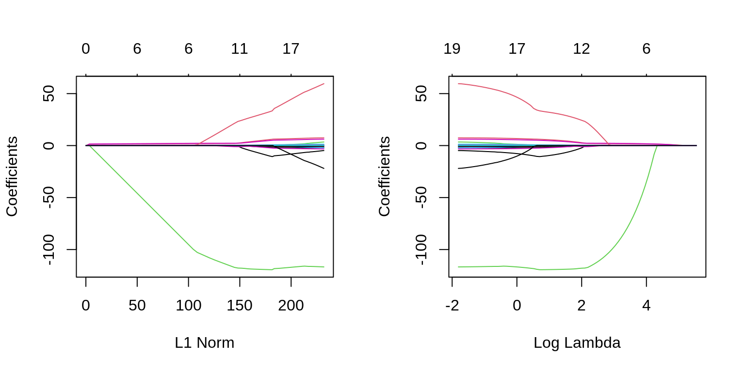
Again, to actually pick a \(\lambda\), we will use cross-validation. The plot is similar to the ridge plot. Notice along the top is the number of features in the model. (Which changed in this plot.)
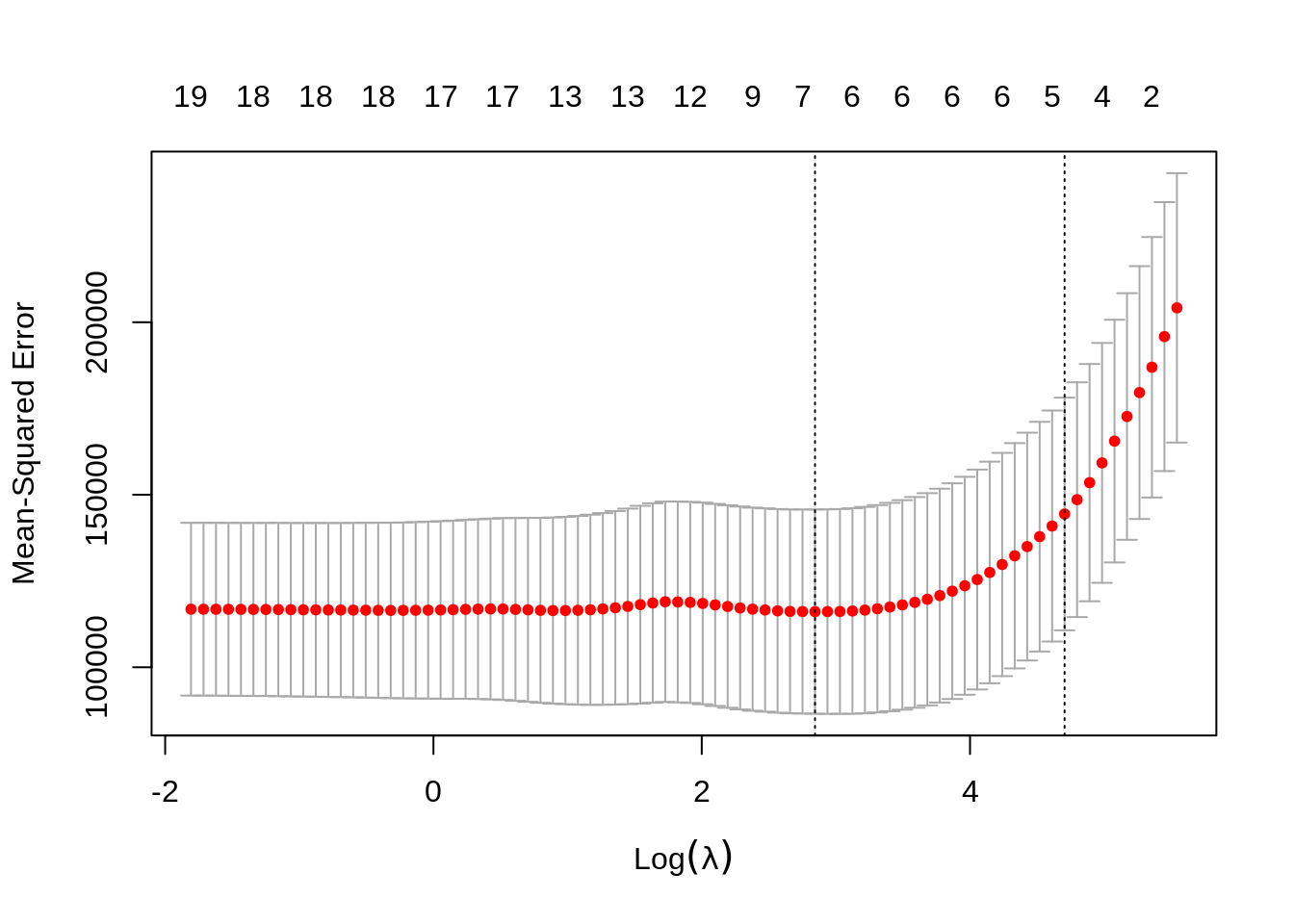
cv.glmnet() returns several details of the fit for both \(\lambda\) values in the plot. Notice the penalty terms are again smaller than the full linear regression. (As we would expect.) Some coefficients are 0.
## 20 x 1 sparse Matrix of class "dgCMatrix"
##                       1
## (Intercept) 251.4491565
## AtBat         .
## Hits          1.0036044
## HmRun         .
## Runs          .
## RBI           .
## Walks         0.9857987
## Years         .
## CAtBat        .
## CHits         .
## CHmRun        .
## CRuns         0.1094218
## CRBI          0.2911570
## CWalks        .
## LeagueN       .
## DivisionW     .
## PutOuts       .
## Assists       .
## Errors        .
## NewLeagueN .## 20 x 1 sparse Matrix of class "dgCMatrix"
## 1
## (Intercept) 20.9671791
## AtBat .
## Hits 1.8647356
## HmRun .
## Runs .
## RBI .
## Walks 2.2144706
## Years .
## CAtBat .
## CHits .
## CHmRun .
## CRuns 0.2067687
## CRBI 0.4123098
## CWalks .
## LeagueN 0.8359508
## DivisionW -102.7759368
## PutOuts 0.2197627
## Assists .
## Errors .
## NewLeagueN .## [1] 10572.23## 20 x 1 sparse Matrix of class "dgCMatrix"
## 1
## (Intercept) 251.4491565
## AtBat .
## Hits 1.0036044
## HmRun .
## Runs .
## RBI .
## Walks 0.9857987
## Years .
## CAtBat .
## CHits .
## CHmRun .
## CRuns 0.1094218
## CRBI 0.2911570
## CWalks .
## LeagueN .
## DivisionW .
## PutOuts .
## Assists .
## Errors .
## NewLeagueN .## [1] 2.075766## [1] 134647.7## [1] 204170.8 195843.9 186963.3 179622.0 172688.0 165552.2 159227.8 153508.8
## [9] 148571.9 144422.7 140935.6 137857.2 134976.5 132308.5 129776.3 127472.4
## [17] 125422.6 123615.4 122061.6 120771.5 119696.7 118804.2 118063.8 117451.0
## [25] 116946.3 116563.7 116300.4 116170.3 116132.8 116127.2 116149.0 116183.0
## [33] 116349.2 116600.5 116841.5 117174.1 117598.5 118064.5 118494.5 118796.4
## [41] 118929.0 118976.5 118618.7 118138.5 117636.1 117229.2 116903.9 116659.7
## [49] 116511.3 116429.7 116433.4 116496.7 116635.7 116759.7 116884.4 116892.4
## [57] 116844.4 116781.5 116684.3 116606.2 116552.0 116510.0 116482.6 116475.8
## [65] 116499.1 116537.0 116558.3 116586.5 116598.2 116638.3 116645.8 116686.1
## [73] 116722.1 116751.7 116760.4 116771.7 116792.0 116806.0 116816.9 116825.5## [1] 116127.212.3 broom
Sometimes, the output from glmnet() can be overwhelming. The broom package can help with that.
library(broom)
# the output from the commented line would be immense
# fit_lasso_cv
tidy(fit_lasso_cv)
## # A tibble: 80 x 6
## lambda estimate std.error conf.low conf.high nzero
## <dbl> <dbl> <dbl> <dbl> <dbl> <int>
## 1 255. 204171. 39048. 165123. 243219. 0
## 2 233. 195844. 38973. 156870. 234817. 1
## 3 212. 186963. 37751. 149212. 224714. 2
## 4 193. 179622. 36640. 142982. 216262. 2
## 5 176. 172688. 35736. 136952. 208424. 3
## 6 160. 165552. 35177. 130376. 200729. 4
## 7 146. 159228. 34767. 124461. 193995. 4
## 8 133. 153509. 34383. 119126. 187892. 4
## 9 121. 148572. 34027. 114545. 182599. 4
## 10 111. 144423. 33723. 110699. 178146. 4
## # … with 70 more rows## # A tibble: 1 x 3
## lambda.min lambda.1se nobs
## <dbl> <dbl> <int>
## 1 17.2 111. 26312.4 Simulated Data, \(p > n\)
Aside from simply shrinking coefficients (ridge and lasso) and setting some coefficients to 0 (lasso), penalized regression also has the advantage of being able to handle the \(p > n\) case.
set.seed(1234)
n = 1000
p = 5500
X = replicate(p, rnorm(n = n))
beta = c(1, 1, 1, rep(0, 5497))
z = X %*% beta
prob = exp(z) / (1 + exp(z))
y = as.factor(rbinom(length(z), size = 1, prob = prob))
We first simulate a classification example where \(p > n\).
We then use a lasso penalty to fit penalized logistic regression. This minimizes
\[ \sum_{i=1}^{n} L\left(y_i, \beta_0 + \sum_{j=1}^{p} \beta_j x_{ij}\right) + \lambda \sum_{j=1}^{p} |\beta_j| \]
where \(L\) is the appropriate negative log-likelihood.
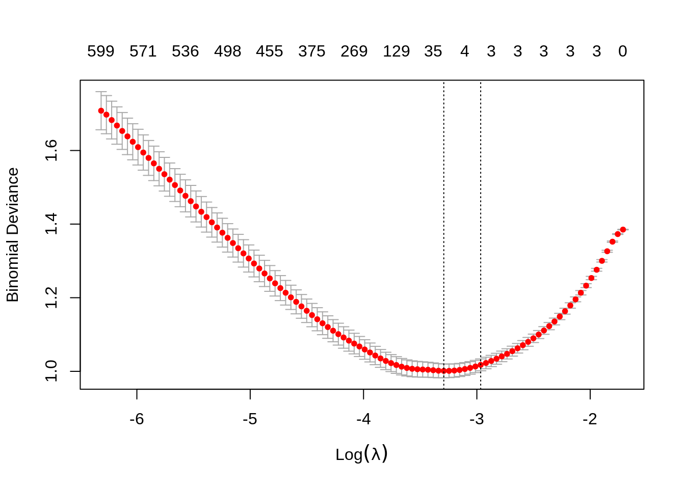
We’re being lazy again and using the entire dataset as the training data.
## 10 x 1 sparse Matrix of class "dgCMatrix"
##                      1
## (Intercept) 0.02397452
## V1          0.59674958
## V2          0.56251761
## V3          0.60065105
## V4          .
## V5          .
## V6          .
## V7          .
## V8          .
## V9 .## s0 s1 s2 s3 s4 s5 s6 s7 s8 s9 s10 s11 s12 s13 s14 s15 s16 s17 s18 s19
## 0 2 3 3 3 3 3 3 3 3 3 3 3 3 3 3 3 3 3 3
## s20 s21 s22 s23 s24 s25 s26 s27 s28 s29 s30 s31 s32 s33 s34 s35 s36 s37 s38 s39
## 3 3 3 3 3 3 3 3 3 3 4 6 7 10 18 24 35 54 65 75
## s40 s41 s42 s43 s44 s45 s46 s47 s48 s49 s50 s51 s52 s53 s54 s55 s56 s57 s58 s59
## 86 100 110 129 147 168 187 202 221 241 254 269 283 298 310 324 333 350 364 375
## s60 s61 s62 s63 s64 s65 s66 s67 s68 s69 s70 s71 s72 s73 s74 s75 s76 s77 s78 s79
## 387 400 411 429 435 445 453 455 462 466 475 481 487 491 496 498 502 504 512 518
## s80 s81 s82 s83 s84 s85 s86 s87 s88 s89 s90 s91 s92 s93 s94 s95 s96 s97 s98 s99
## 523 526 528 536 543 550 559 561 563 566 570 571 576 582 586 590 596 596 600 599Notice, only the first three predictors generated are truly significant, and that is exactly what the suggested model finds.
fit_1se = glmnet(X, y, family = "binomial", lambda = fit_cv$lambda.1se)
which(as.vector(as.matrix(fit_1se$beta)) != 0)
## [1] 1 2 3We can also see in the following plots, the three features entering the model well ahead of the irrelevant features.
par(mfrow = c(1, 2))
plot(glmnet(X, y, family = "binomial"))
plot(glmnet(X, y, family = "binomial"), xvar = "lambda")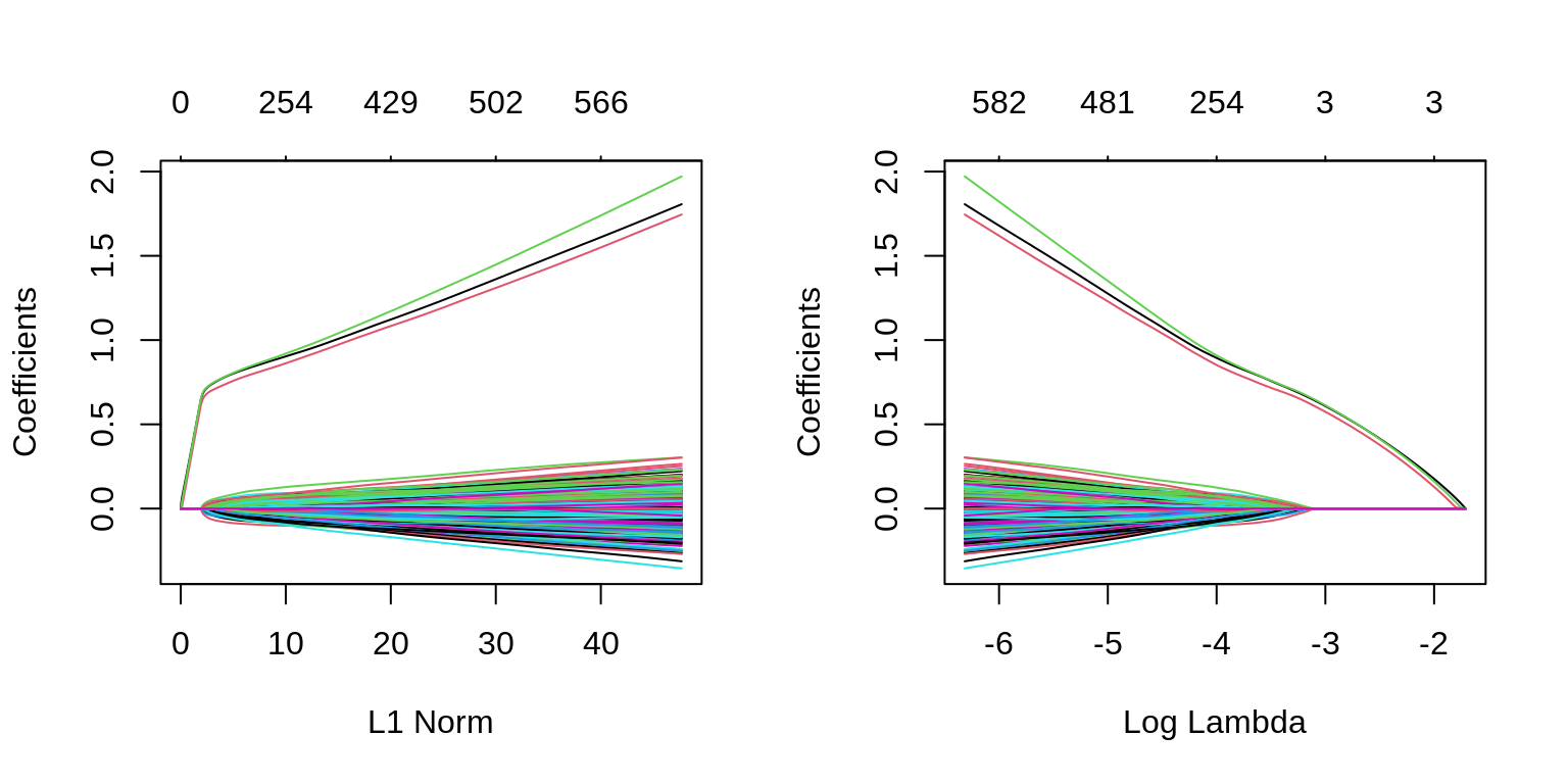
We can extract the two relevant \(\lambda\) values.
## [1] 0.03718493## [1] 0.0514969TODO: use default of type.measure="deviance" but note that type.measure="class" exists.