D Statistics
STAT 432 is a course about statistics, in particular, some specific statistics. To discuss the statistics of interest in STAT 432, we will need some general concepts about statistics.
D.1 Reading
- Reference: STAT 400 @ UIUC: Notes and Homework
- Reference: STAT 3202 @ OSU: Fitting a Probability Model
- Reference: STAT 415 @ PSU: Notes
D.2 Statistics
In short: a statistic is a function of (sample) data. (This mirrors parameters being functions of (population) distributions. In SAT terminology, statistics : data :: parameter : distribution.)
Consider a random variable \(X\), with PDF \(f(x)\) which defines the distribution of \(X\). Now consider the parameter \(\mu\), which we usually refer to as the mean of a distribution. We use \(\mu_X\) to note that \(\mu\) is dependent on the distribution of \(X\).
\[ \mu_X = \text{E}[X] = \int_{-\infty}^{\infty}xf(x)dx \]
Note that this expression is a function of \(f(x)\). When we change the distribution of \(X\), that is, it has a different \(f(x)\), that effects \(\mu\).
Now, given a random sample \(X_1, X_2, \ldots, X_n\), define a statistic,
\[ \hat{\mu}(x_1, x_2, \ldots, x_n) = \frac{1}{n}\sum_{i = 1}^{n}x_i \]
Often, we will simplify notation and instead simply write
\[ \hat{\mu} = \frac{1}{n}\sum_{i = 1}^{n}x_i \]
and the fact that \(\hat{\mu}\) is a function of the sample is implied. (You might also notice that this is the sample mean, which is often denoted by \(\bar{x}\).)
Another confusing aspect of statistics is that they are random variables! Sometimes we would write the above as
\[ \hat{\mu}(X_1, X_2, \ldots, X_n) = \frac{1}{n}\sum_{i = 1}^{n}X_i \]
When written this way, we are emphasizing that the random sample has not yet be observed, thus is still random. When this is the case, we can investigate the properties of the statistic as a random variable. When the sample has been observed, we use \(x_1, x_2, \ldots, x_n\) to note that we are inputting these observed values into a function, which outputs some value. (Sometimes we, and others, will be notationally sloppy and simply use lower case \(x\) and you will be expected to understand via context if we are dealing with random variables or observed values of random variables. This is admittedly confusing.)
As a final note, suppose we observe some data
\[ x_1 = 2, x_2 = 1, x_3 =5 \]
and we calculate \(\hat{\mu}\) given these values. We would obtain
\[ \hat{\mu} = \frac{8}{3} \approx 2.66 \]
Note that 2.66 is not a statistic. It is the value of a statistic given a particular set of data. The statistic is still \(\hat{\mu}\) which has output the value 2.66. Statistics output values given some data.
D.3 Estimators
Estimators are just statistics with a purpose, that is, estimators are statistics that attempt to estimate some quantity of interest, usually some parameter. (In other words, learn from data.) Like statistics, estimators are functions of data that output values, which we call estimates.
D.3.1 Properties
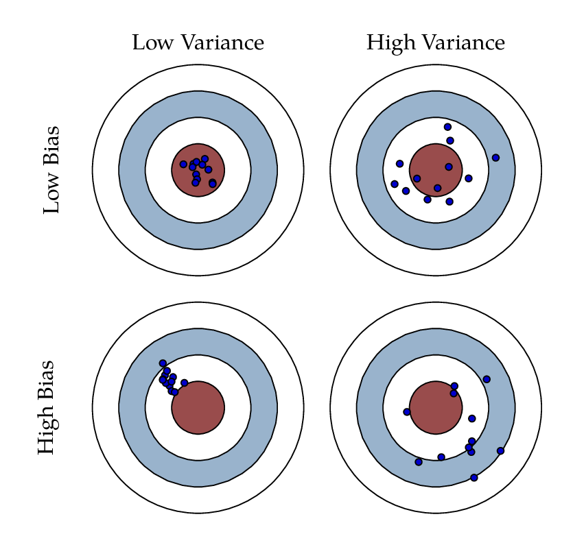
Bias and Variance Visually Illustrated
Because they are just statistics, estimators are simply functions of data. What makes an estimator good? Essentially, an estimator is good if it produces estimates that are close to the thing being estimated. The following properties help to better define this “closeness” as a function of the errors made by estimators.
To estimate some parameter \(\theta\) we will consider some estimator \(\hat{\theta}\).
D.3.1.1 Bias
The bias of an estimator defines the systematic error of the estimator, that is, how the estimator “misses” on average.
\[ \text{bias}\left[\hat{\theta}\right] \triangleq \mathbb{E}\left[\hat{\theta}\right] - \theta \]
D.3.1.2 Variance
The variance of an estimator defines how close resulting estimates are to each other. (Assuming the estimated was repeated.)
\[ \text{var}\left[\hat{\theta}\right] \triangleq \mathbb{E}\left[ \left( \hat{\theta} - \mathbb{E}\left[\hat{\theta}\right] \right)^2 \right] \]
D.3.1.3 Mean Squared Error
The mean squared error (MSE) is exactly what the name suggests, it is the average squared error of the estimator. Interestingly, the MSE decomposes into terms related to the bias and the variance. We will return to this idea later for a detailed discussion in the context of machine learning.
\[ \text{MSE}\left[\hat{\theta}\right] \triangleq \mathbb{E}\left[\left(\hat{\theta} - \theta\right)^2\right] = \left(\text{bias}\left[\hat{\theta}\right]\right)^2 + \text{var}\left[\hat{\theta}\right] \]
D.3.1.4 Consistency
An estimator \(\hat{\theta}_n\) is said to be a consistent estimator of \(\theta\) if, for any positive \(\epsilon\),
\[ \lim_{n \rightarrow \infty} P\left( \left| \hat{\theta}_n - \theta \right| \leq \epsilon\right) =1 \]
or, equivalently,
\[ \lim_{n \rightarrow \infty} P\left( \left| \hat{\theta}_n - \theta \right| > \epsilon\right) =0 \]
We say that \(\hat{\theta}_n\) converges in probability to \(\theta\) and we write \(\hat{\theta}_n \overset P \rightarrow \theta\).
D.3.2 Example: MSE of an Estimator
Consider \(X_1, X_2, X_3 \sim N(\mu, \sigma^2)\).
Define two estimators for the true mean, \(\mu\).
\[ \bar{X} = \frac{1}{n}\sum_{i = 1}^{3} X_i \]
\[ \hat{\mu} = \frac{1}{4}X_1 + \frac{1}{5}X_2 + \frac{1}{6}X_3 \]
We will now calculate and compare the mean squared error of both \(\bar{X}\) and \(\hat{\mu}\) as estimators of \(\mu\).
First, recall from properties of the sample mean that
\[ \text{E}\left[\bar{X}\right] = \mu \]
and
\[ \text{var}\left[\bar{X}\right] = \frac{\sigma^2}{3} \]
Thus we have
\[ \text{bias}\left[\bar{X}\right] = \mathbb{E}\left[\bar{X}\right] - \mu = \mu - \mu = 0 \]
Then,
\[ \text{MSE}\left[\bar{X}\right] \triangleq \left(\text{bias}\left[\bar{X}\right]\right)^2 + \text{var}\left[\bar{X}\right] = 0 + \frac{\sigma^2}{3} = \frac{\sigma^2}{3} \]
Next,
\[ \text{E}\left[\hat{\mu}\right] = \frac{\mu}{4} + \frac{\mu}{5} + \frac{\mu}{6} = \frac{37}{60}\mu \]
and
\[ \text{var}\left[\hat{\mu}\right] = \frac{\sigma^2}{16} + \frac{\sigma^2}{25} + \frac{\sigma^2}{36} = \frac{469}{3600}\sigma^2 \]
Now we have
\[ \text{bias}\left[\hat{\mu}\right] = \mathbb{E}\left[\hat{\mu}\right] - \mu = \frac{37}{60}\mu - \mu = \frac{-23}{60}\mu \]
Then finally we obtain the mean squared error for \(\hat{\mu}\),
\[ \text{MSE}\left[\hat{\mu}\right] \triangleq \left(\text{bias}\left[\hat{\mu}\right]\right)^2 + \text{var}\left[\hat{\mu}\right] = \left( \frac{-23}{60}\mu \right)^2 + \frac{469}{3600}\sigma^2 \]
Note that \(\text{MSE}\left[\hat{\mu}\right]\) is small when \(\mu\) is close to 0.
D.3.3 Estimation Methods
So far we have discussed properties of estimators, but how do we create estimators? You could just define a bunch of estimators and then evaluate them to see what works best (an idea we will return to later in the context of ML) but (the field of) statistics has develop some methods that result in estimators with desirable properties.
D.3.4 Maximum Likelihood Estimation
Given a random sample \(X_1, X_2, \ldots, X_n\) from a population with parameter \(\theta\) and density or mass \(f(x; \theta)\), we define the likelihood as
\[ \mathcal{L}(\theta \mid x_1, x_2, \ldots x_n) \triangleq f(x_1, x_2, \ldots, x_n; \theta) = \prod_{i = 1}^n f(x_i; \theta) \]
The Maximum Likelihood Estimator, \(\hat{\theta}\)
\[ \hat{\theta} \triangleq \underset{\theta}{\text{argmax}} \ \mathcal{L}(\theta \mid x_1, x_2, \ldots x_n) = \underset{\theta}{\text{argmax}} \ \log \mathcal{L}(\theta \mid x_1, x_2, \ldots x_n) \]
D.3.4.1 Invariance Principle
If \(\hat{\theta}\) is the MLE of \(\theta\) and the function \(h(\theta)\) is continuous, then \(h(\hat{\theta})\) is the MLE of \(h(\theta)\).
D.3.5 Method of Moments
While it is very unlikely that we will use the Method of Moments in STAT 432, you should still be aware of its existence.
D.3.6 Empirical Distribution Function
Consider a random variable \(X\) with CDF \(F(k) = P(X < k)\) and an iid random sample \(X_1, X_2, \ldots, X_n\). We can estimate \(F(k)\) using the Empirical Distribution Function (EDF),
\[ \hat{F}(k) = \frac{\text{# of elements in sample} \leq k}{n} = \frac{1}{n} \sum_{i = 1}^n I(x_i \leq k) \]
where \(I(x_i \leq k)\) is an indicator such that
\[ I(x_i \leq k) = \begin{cases} 1 & \text{if } x_i \leq k \\ 0 & \text{if } x_i > k \end{cases} \]
Given a data vector in R that is assumed to be a random sample, say, y, and some value, say k, it is easy to calculate \(\hat{F}(k)\).
set.seed(66)
y = rnorm(n = 25, mean = 6, sd = 2.6) # generate sample
k = 4 # pick some k
head(y) # check data
## [1] 12.042334 6.564140 7.087301 5.503419 5.181420 4.315569## [1] 0.2# using an estimated normal distribution (not quite using the MLE)
pnorm(q = k, mean = mean(y), sd = sd(y))## [1] 0.2088465## [1] 0.2208782Note that technically sd(x) does not return the MLE of \(\sigma\) since it uses the unbiased estimator with a denominator of \(n - 1\) instead of \(n\), but we’re being lazy for the sake of some cleaner code.
plot(ecdf(y),
     col.01line = "white", verticals = TRUE, do.points = FALSE,
     xlim = c(0, 15), lwd = 2, lty = 1, ylab = "F(y)", xlab = "y",
     main = "Comparing the EDF to The Truth and MLE")
curve(pnorm(x, mean = 6, sd = 2.6),
      add = TRUE, xlim = c(0, 15), col = "dodgerblue", lty = 2, lwd = 2)
curve(pnorm(x, mean = mean(y), sd = sd(y)),
      add = TRUE, xlim = c(0, 15), col = "darkorange", lty = 3, lwd = 2)
legend("bottomright", legend = c("EDF", "Truth", "MLE"),
  col = c("black", "dodgerblue", "darkorange"), lty = 1:3, lwd = 2)
grid()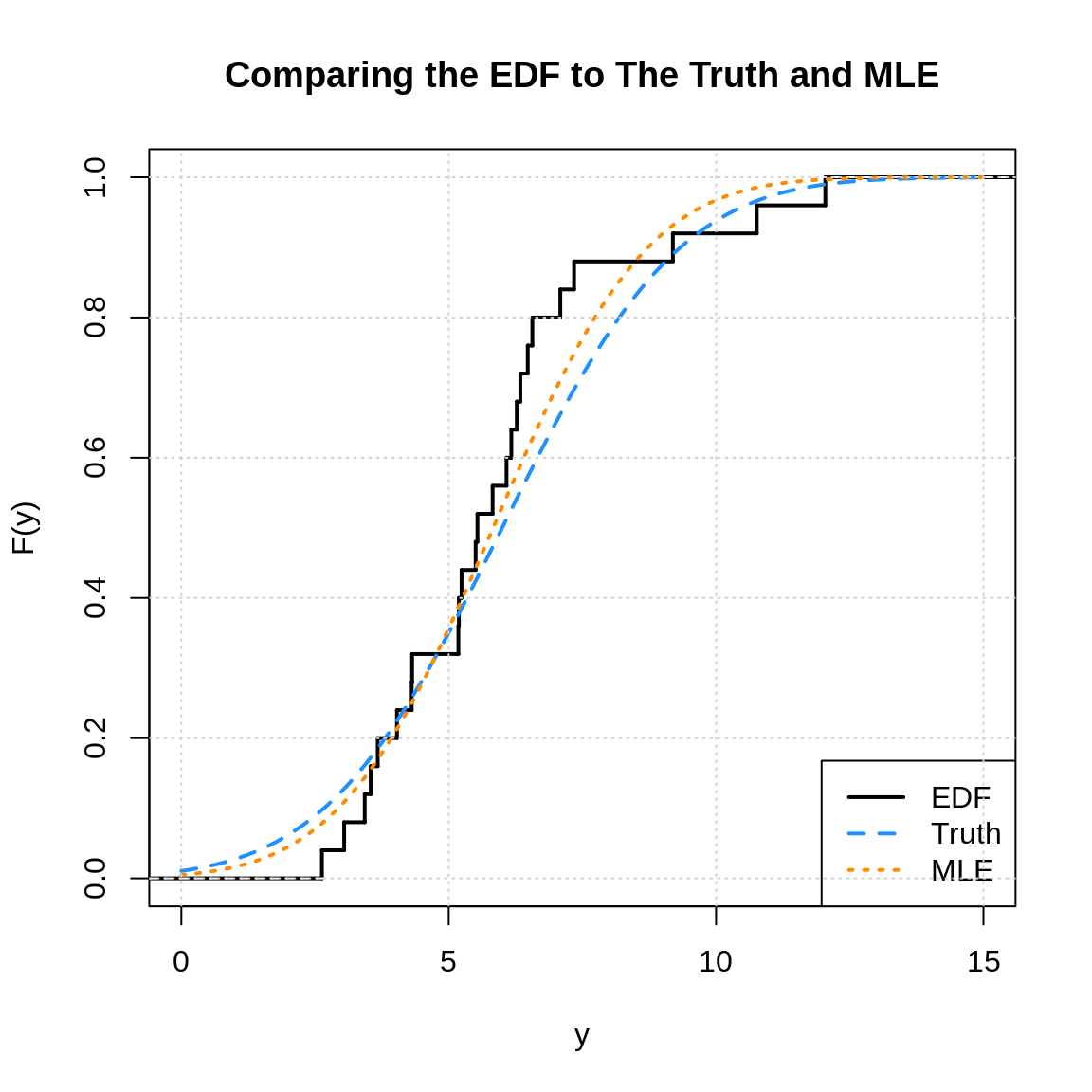
We have purposefully used a “small” sample size here so that the EDF is visibly a step function. Modify the code above to increase the sample size. You should notice that the three functions converge as the sample size increases.